Severe Convective Storms have become the largest driver of insured losses in the United States. As carriers and reinsurers push for better understanding of hail, straight-line wind, and tornado risk, the pressure to evaluate SCS models rigorously has never been higher.
Yet many common validation strategies, using hail days, relying on raw SPC storm reports, or comparing county-wide maximum wind gusts to grid-cell model output, create the illusion of insight while introducing significant bias.
This article breaks down a scientifically robust method for how KatRisk views SCS model evaluation, which metrics mislead more than they illuminate, and why scientifically grounded validation matters more than ever.
Why Many SCS Validation Methods Are Misleading From the Start
What often looks like model underperformance is simply misinterpreted data — and it comes down to three predictable pitfalls embedded in surface-station wind observations.
Pitfall #1 — Treating Raw Wind Observations as “Ground Truth”
ASOS/AWOS weather stations are essential for meteorology — but they are not designed for catastrophe-model validation. They frequently include:
- Tornado gusts misclassified as straight-line wind
- Instrument or reporting errors
- Non-representative extremes driven by storm structure
- Large spatial inconsistencies during the same event
A single example reveals the stakes.
Case Study: The “100-Year” Wind Gust That Was Actually a Tornado
In 2013, the Denver International Airport ASOS station recorded a 97-mph gust, well above the KatRisk 100-year straight-line wind return period for the location.
On paper, this looks like significant model underestimation.
In reality, a tornado passed directly over the station on 18 June 2013. The gust was not a straight-line wind event at all and thus not representative of straight-line wind climate.
This type of misclassification happens frequently and dramatically skews any validation that blindly uses station maxima.
Pitfall #2 — Not Accounting for Known ASOS Errors
Surface stations produce well-documented spurious readings:
- Luke Air Force Base in Maricopa County reported a 102-mph gust on 5 May 2009 on a day with no thunderstorms anywhere in the region.
- SPC routinely corrects ASOS reports through expert quality control. For example, an 88-mph gust at Gila AFB on 30 July 2016 was revised to 77 mph to match observed regional reality.
Standard ASOS wind measurement error is also roughly 5 percent (NOAA, 1998).
Why comparing to county-wide maxima is flawed
Maricopa County illustrates the mismatch:
- One station measured 77 mph
- Another measured 25 mph
- The median gust across all stations was 48 mph
The county maximum is often 65 percent higher than the minimum and 24 percent higher than the median, not because the model is wrong, but because the storm environment is spatially variable.
Catastrophe models simulate hazard at the grid-cell level. They should be validated against point-level observations, not against the highest observation from a wide geographic area.
Proper validation: Use individual station data
When station-level annual maxima are compared to KatRisk return periods, they:
- Align closely with the KatRisk 10-year and 100-year estimates
- Only rarely exceed return periods, at frequencies expected by probability theory
- Exhibit about a 20 percent chance of exceeding a 100-year gust over 2000–2023
This is the correct spatial scale for validation.
Pitfall #3 — Surface Stations are Spaced too far Apart
ASOS stations are typically located at airports, leaving most metros only 1-2 stations and most rural areas without any stations. Some state and private entities maintain higher-density surface station networks (i.e., mesonets), but at best they are spaced tens of kilometers apart and are not necessarily as accurate.
Since the surface stations are spaced far apart, they often are unable to observe the most intense wind gusts in a thunderstorm. These wind gusts are small in scale and occur over short time windows. For example:
- A derecho hit downtown Houston on May 16 2024, post-event damage surveys conducted by the National Weather Service suggested wind gusts exceeded 100 mph
- Surface stations within and surrounding downtown Houston reported 60-70 mph wind gusts, 30-40 mph below peak wind gust estimates.
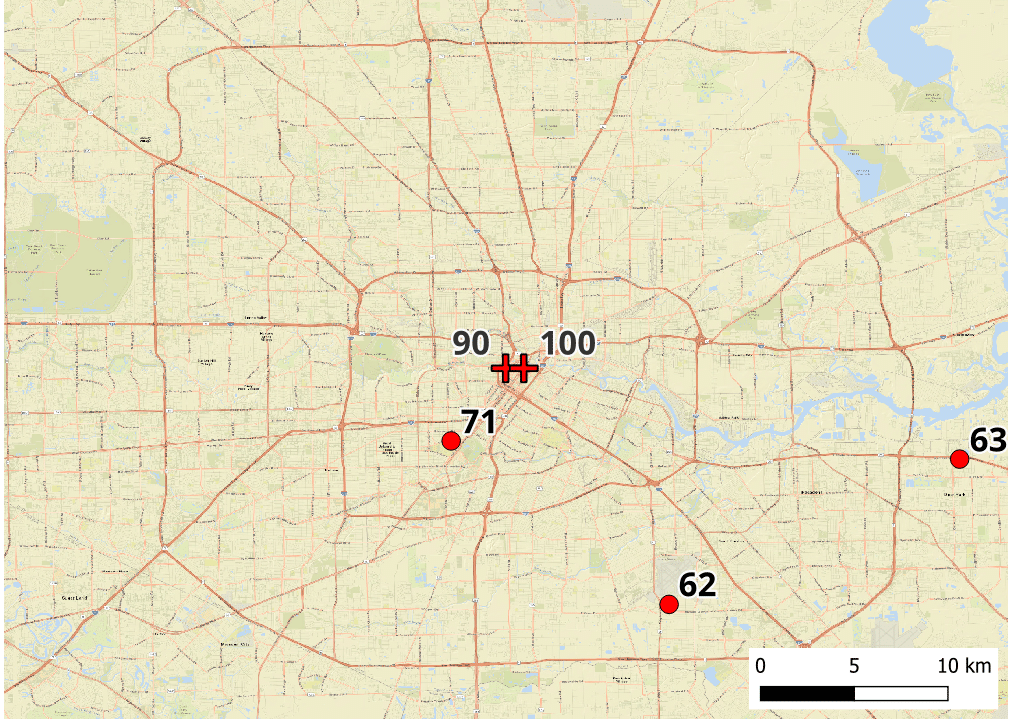
A map of the surface station reported peak wind gusts (circles) during the May 16 Houston derecho. National Weather Service post-event storm damage survey wind speed estimates are marked with plus signs. Wind gusts are in mph.
ASOS stations provide timely wind speed observations for a given location. However, even in densely populated areas, they are unable to regularly observe event peak wind gusts over a larger region.
Why “Hail Days” Can be a Misleading Validation Metrics
“Hail days” — the number of days per year with ≥1″ hail reports, is one of the most widely used but fundamentally biased validation metrics in the industry. The reasons are structural, statistical, and observational.
Problem #1 — The SPC Database Has Structural Shifts Over Time
The SPC Storm Reporting Database is widely used but contains major long-term discontinuities that make simple trend comparisons misleading. Key changes include:
- Early 1990s — Doppler radar deployment
More weak tornadoes were detected, increasing tornado report counts. - 1990s — Rise in public reporting
More people began submitting severe weather observations, increasing report volume regardless of actual hazard. - 2007 — Adoption of the Enhanced Fujita (EF) Scale
Wind speeds associated with tornado intensity shifted due to the new classification system. - 2010 — Severe hail threshold increased from 0.75″ to 1.00″
After this change, far fewer 0.75″ reports and far more 1.00″ reports appeared — even though the storms themselves did not change.
Any validation using SPC reports before and after these shifts must explicitly account for these artificial jumps.
Problem #2 — Hail Reporting Is Dominated by Household-Object Estimates
People rarely measure hailstones directly. Instead they compare them to familiar objects:
- Penny (0.75″)
- Nickel (0.88″)
- Quarter (1.00″)
- Golf ball (1.75″)
These four bins account for 84 percent of all SPC hail reports.
This clustering is a reporting artifact, not meteorology.
Threshold sensitivity: 1.00″ vs. 1.75″ vs. 2.00″
A subtle but important nuance: the number of hail days does not always decrease when increasing the hail size threshold. For example:
- The number of hail days is often identical when comparing 1.80″ vs. 2.00″.
Why?
Because SPC only reports certain discrete sizes (0.75, 0.88, 1.00, 1.25, 1.50, 1.75, 2.00).
All hail between 1.76″ and 2.00″ gets lumped into the 2.00″ bin.
This makes hail day counts extremely non-continuous and therefore unstable.
Problem #3 — Small, Low-Loss Events Dominate the Hail Day Count
Hail days are often driven by marginal, small-footprint events that:
- Occur under weak instability
- Produce small hailstones
- Cover little area
- Contribute negligible insured loss
When filtering to exclude these small events (requiring reports in at least four 0.25° grid cells — roughly county scale):
- Hail days drop by 35–40 percent in the Plains
When also removing hailstones ≤1″, the total drops by 60 percent in many regions.
This demonstrates that the “hail day” metric is disproportionately influenced by noise, low-impact reports, and small storms that do not drive loss.
Better Ways to Evaluate an SCS Model
To properly evaluate an SCS model, focus on metrics tied to physical realism, hazard behavior, and loss generation.
- Hail size distributions, not hail-day counts – Compare modeled hail size frequencies to research-grade datasets (e.g., Ortega, Blair), not uncalibrated public reports.
- Event-scale hazard structure – Assess swath continuity, spatial extent, and intensity gradients.
- Point-based return period comparisons– Use individual station annual maxima for straight-line wind analyses — not county maxima.
- Event frequency vs. loss-driving frequency – Distinguish between marginal hailstorms and large, damaging hail events.
- Consistency under correlation sensitivity – Test how small changes to spatial correlation affect hail footprint counts.
- Loss validation – Compare modeled and historical loss ratios, footprint severity, and event clustering.
These approaches test what actually drives carrier outcomes — not what happens when the public mistakes a nickel for a quarter.
Key Takeaways for SCS Model Buyers and Validators
Accurate SCS model evaluation requires more than simple observational metrics. Users must understand the limitations of SPC reports, ASOS reliability, hail size clustering, threshold discontinuities, and spatial sampling biases
- Avoid hail days as a primary validation metric — the dataset is unstable, clustered, threshold-sensitive, and dominated by marginal events.
- Do not rely on unfiltered SPC or ASOS data — tornado contamination, reporting bias, and spatial sampling inconsistencies distort results.
- Validate at the correct spatial scale — point-level observations should be compared to point-level model output.
- Evaluate hazard realism, not superficial report counts — insurer losses come from large, spatially coherent hail and wind events.
- Understand SPC database evolution — structural changes in 1990s, 2007, and 2010 create artificial trends that must be accounted for.
KatRisk’s SCS model is designed around high-resolution hazard simulation, scientifically grounded spatial correlation, and rigorous multi-scale validation. By focusing on the metrics that actually capture hazard and loss, rather than easily distorted report counts, users can select and trust models that hold up under scrutiny.